") の形で表されているときの積分値を求める
の形で表されているときの積分値を求める
(1)「電気・電子工学のための数値計算法入門」橋本修著 総合電子出版社
(2)「ディジタル信号処理技術」玉井徳みち、長島厚、藤田泰弘、若井修造著 日経BP社
(3)「よくわかる有限要素法」福森栄次著 Ohmsha
http://szksrv.isc.chubu.ac.jp/java/physics/rlc/rlc0.html
http://www.asahi-net.or.jp/~jk2m-mrt/kiso_RLC.htm
http://ja.wikipedia.org/wiki/%E4%B8%89%E8%A7%92%E9%96%A2%E6%95%B0
http://www.cmplx.cse.nagoya-u.ac.jp/~furuhashi/education/CircuitMaker/chap1.pdf
http://www.akita-nct.ac.jp/~yamamoto/lecture/2003/5E/lecture_5E/diff_eq/node2.html
http://chemeng.on.coocan.jp/cemath/cemath08.html
http://homepage3.nifty.com/skomo/f6/hp6_3.htm
http://homepage1.nifty.com/gfk/rungekutta.htm
(a) 微分の説明
微分方程式の解を求める
(b) 微分方程式の解を数値計算で求める
(c) 積分の説明
(d) 関数が微分の形の形で表されているときの積分値を求める
(一般的に数値積分をする意味は、関数自体が変化の式(例えば速度の関数)などで表されているとき
ある時刻から時刻までの距離を求めたいときなどで使用される。
もちろんその変化の式が、手計算によって計算可能ならば積分によって時間と距離の関係を導出し
その時間を入れることで直接距離を導いたほうが早い。
しかし、一般的に時間と距離の関係のような式自体が導出することが不可能な場合が世の中には多く
時間と速度の関係のような変化の式を見つけ出すことの方が容易なのだが、これを手計算で積分すること
は非常に難しいため数値積分が提案された)
(☆)注意 微分方程式の解を求めるのであって、微分するのではない。
つまり、微係数を求めるのではない
ある連続関数") ,
,  において、区間[a,b]をn等分し、その間隔を
 とする。
とする。
_i = \frac{ y_{i+1} - y_{i} }{h}")
の_i \times h + y_{i}")
の を求めるのが常微分方程式の解を求める作業。
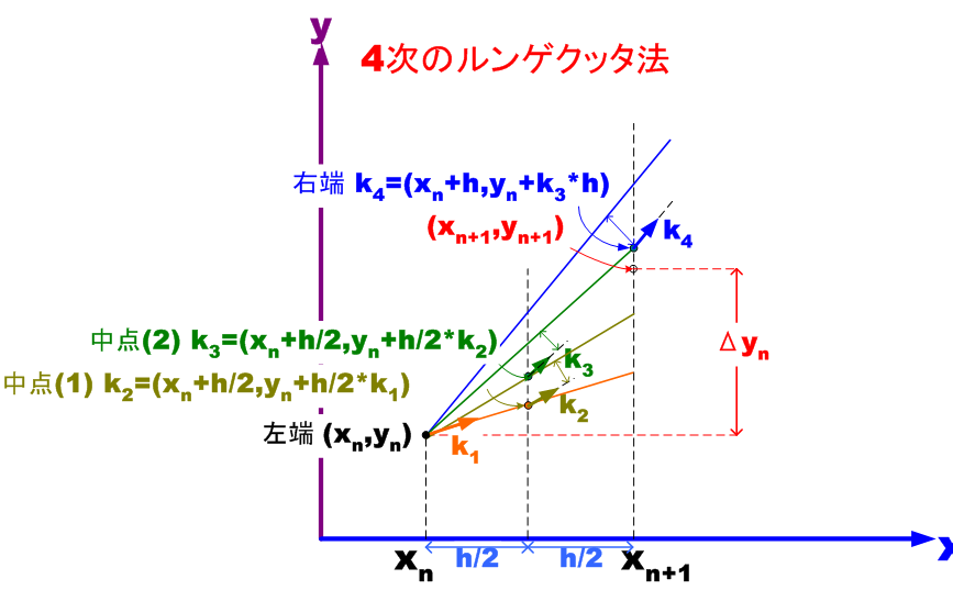
微分方程式の初期解を求める方法として、ルンゲクッタ法を説明する。
ルンゲクッタ法を簡単にいえば、適切な傾き(微係数)を求めて") と傾きおよび
と傾きおよび までの距離から
 を求めることである。
解法を以下に説明する。
(1) オレンジ色の直線の微分は、点 の微分なので、
 での微係数は、
=f(x_n , y_n )") (1-1)となる。
(1-1)となる。
(2-a) 幅h/2の間、yの関数の傾きは,") であったと仮定して、
であったと仮定して、") の値を仮定する。
の値を仮定する。
=k1(n)*( \frac{h}{2}) + y_n")
そうすると、)") の微係数は、
の微係数は、
=f(x_n+\frac{h}{2},y_n+\frac{h}{2}*k1(n))") (1-2)
(1-2)
(2-b) 次に再び幅h/2の間、yの関数の傾きは,") であったと仮定すると
であったと仮定すると
=k2(n)*( \frac{h}{2}) + y_n")
そうすると、)") の微係数は、
の微係数は、
=f(x_n+\frac{h}{2},y_n+\frac{h}{2}*k2(n))") (1-3)
(1-3)
次にこの傾きが十分に正しいと仮定して、実際に のときの
のときの を求めてみる。
=k3(n)*(h) + y_n")
そうすると、)") の微係数は、
の微係数は、
=f(x_n+h,y_n + k3(n)*h)") (1-4)
(1-4)
この4つの微係数に1:2:2:1の重みをかけて6で割った微係数にhをかけることで は求められる。
 + 2k2(n) + 2k3(n) + k4(n) )*h") (1-5)
(1-5)
=f(x_n , y_n )") (1-1)
(1-1)=f(x_n+\frac{h}{2},y_n+\frac{h}{2}*k1(n))") (1-2)
(1-2)=f(x_n+\frac{h}{2},y_n+\frac{h}{2}*k2(n))") (1-3)
(1-3)=f(x_n+h,y_n + k3(n)*h)") (1-4)
(1-4)
 + 2k2(n) + 2k3(n) + k4(n) )*h") (1-5)
(1-5)
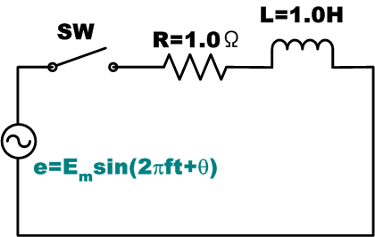
}{dt} + Ri(t) = E\sin(\omega t)") ときの解
ときの解
は、
") (A-1)
(A-1)
となるので = \frac{R}{L}")
 = \frac{E}{L}\sin(\omega t)")

となる。}") とおいて変数変換すると
とおいて変数変換すると
P(x)u = (1-n)Q(x)")
") (A-2)
(A-2)
") が0のときの解をまず考える(過度解)
が0のときの解をまず考える(過度解)


両辺を積分すれば、


ここで とすれば、
とすれば、
この方程式の解は
 (A-3)
(A-3)
( は0を含む任意の実数)となる。
(A-3)の積分定数Cをxの関数とすると
 (A-4)
(A-4)
(A-4)に(A-2)(A-3)を代入する") (A-2)
(A-2)
\frac{dC}{dt} = \frac{E}{L}\sin(\omega t)")
")
{dt}")
両辺を積分すれば、
{dt}")
{dt}")
{dt}")
は部分分数法で展開できて
{dt}")
'\sin(\omega t){dt}")
 - \int (\frac{\omega L}{R}e^{\frac{R}{L}t})\cos(\omega t){dt}")
 - \frac{\omega L}{R}\int (e^{\frac{R}{L}t})\cos(\omega t){dt}")
次に\cos(\omega t){dt}")
'\cos(\omega t){dt}")
 + \int (\frac{\omega L}{R}e^{\frac{R}{L}t})\sin(\omega t){dt}")
次に{dt}") とおくと
とおくと
 -\frac{\omega L}{R}\Big(\frac{L}{R}e^{\frac{R}{L}t}\cos(\omega t) + \frac{\omega L}{R} I \Big)")
 -\frac{\omega L^2}{R^2}e^{\frac{R}{L}t}\cos(\omega t) - \frac{(\omega L)^2}{R^2} I")
^2}{R^2}I = \frac{L}{R}e^{\frac{R}{L}t}\sin(\omega t) -\frac{\omega L^2}{R^2}e^{\frac{R}{L}t}\cos(\omega t)")
^2}e^{\frac{R}{L}t}\sin(\omega t) -\frac{\omega L^2}{R^2 + (\omega L)^2}e^{\frac{R}{L}t}\cos(\omega t)")
^2}e^{\frac{R}{L}t}\Big( R\sin(\omega t)-\omega L\cos(\omega t)\Big)")
ゆえに
^2}e^{\frac{R}{L}t}\Big( R\sin(\omega t)-\omega L\cos(\omega t)\Big)")
^2}e^{\frac{R}{L}t}\Big( R\sin(\omega t)-\omega L\cos(\omega t)\Big) + D")
( は0を含む任意の実数(積分変数)) (A-5)
(A-2)に(A-5)を代入すると^2}e^{\frac{R}{L}t}\Big( R\sin(\omega t)-\omega L\cos(\omega t)\Big) + D) e^{-\frac{R}{L}t}")
^2}\Big( R\sin(\omega t)-\omega L\cos(\omega t)\Big) + De^{-\frac{R}{L}t}")
}") (3-2)とおいて
(3-2)とおいて なので
なので = \frac{E}{R^2 + (\omega L)^2}\Big( R\sin(\omega t)-\omega L\cos(\omega t)\Big) + De^{-\frac{R}{L}t}")
^2}}\Big( \frac{R}{\sqrt{R^2 + (\omega L)^2}}\sin(\omega t)-\frac{\omega L}{\sqrt{R^2 + (\omega L)^2}}\cos(\omega t)\Big)")
^2}}\Big(\cos(\varphi)\sin(\omega t)-\sin(\varphi)\cos(\omega t)\Big)")
^2}}\Big(\sin(\omega t)\cos(\varphi)-\sin(\varphi)\cos(\omega t)\Big)")
^2}}\sin(\omega t - \varphi)")
ただし、")
ここで、 のとき
のとき=0") の初期条件の元では、
の初期条件の元では、
^2}}\sin(- \varphi)")
^2}}\sin(\varphi)")
^2}}\sin(\varphi)")
= \frac{E}{\sqrt{R^2 + (\omega L)^2}}\sin(\varphi)e^{-\frac{R}{L}t} + \frac{E}{\sqrt{R^2 + (\omega L)^2}}\sin(\omega t - \varphi)")
= \frac{E}{\sqrt{R^2 + (\omega L)^2}}\Big(\sin(\varphi)e^{-\frac{R}{L}t} + \sin(\omega t - \varphi)\Big)")
}{dt} = \frac{\sin(\omega t + \theta) - Ri(t)}{L}")
の = \frac{\sin(\omega t + \theta) - Ri(t)}{L}")
として
=f(t_n , i_n )") (1-1)
(1-1)=f(t_n+\frac{h}{2},i_n+\frac{h}{2}*k_{1}(n))") (1-2)
(1-2)=f(t_n+\frac{h}{2},i_n+\frac{h}{2}*k_{2}(n))") (1-3)
(1-3)=f(t_n+h,i_n + k_{3}(n)*h)") (1-4)
(1-4)
 + 2k_{2}(n) + 2k_{3}(n) + k_{4}(n) )*h") (1-5)
(1-5)
// 4ziRungeKuttaSample.cpp : コンソール アプリケーションのエントリ ポイントを定義します。
//

#include "stdafx.h"
#include<iostream>
#include<fstream>
#include<io.h>
#include<math.h>

#define PI 3.1415926

const static double Em=1.0;                              //電圧源
const static double R=1.0;                               //抵抗
const static double L=1.0;                               //コイル
const static double freq=0.1;                            //周波数0.1Hz
const static double omega=2*PI*freq;                     //角周波数
const static double theta=-PI/4.0;
const static double phi=atan(omega*L/R);
const static double tau = L/R;                           //時定数
const static double dh=(1/freq)/30.;                     //1周期の30分割
const static double Im=1.0/sqrt(R*R+(omega*L)*(omega*L));

double ii4(double t,double cur);

int _tmain(int argc, _TCHAR* argv[])
{

	errno_t err;
	FILE *fp_output;

	//変数
	double t=0;    //実時間
	double e=0; //初期電圧
	double i1=0.0;       //初期電流(厳密解)
	double i4=0.0;       //初期電流(4次のルンゲクッタ法)
	double k[4]={0,0,0,0};

	if( err = fopen_s(&fp_output,"data.txt","w")  != 0){ exit(2);}

	t=0;
	for(int n=1; n< 3*(int)((1/freq)/dh); n++){

		//これは t=n*dh(n=1,2,3,...)の計算となる
		k[0]=ii4(t,i4);
		k[1]=ii4(t+dh/2,i4+dh/2*k[0]);
		k[2]=ii4(t+dh/2,i4+dh/2*k[1]);
		k[3]=ii4(t+dh,i4+dh*k[2]);

		i4=i4+(1./6.)*(k[0]+2*k[1]+2*k[2]+k[3])*dh;

		//n=1から始まるから t=n*dh(n=1,2,3...)
		t=(double)n*dh;

		//電源電圧
		e=Em*sin(omega*t+theta);
		//理論値電流
		i1=Im*(sin(omega*t+theta-phi)-exp(-t/tau)*sin(theta-phi));

		printf("t = %f e=%f i1 = %f i4 = %f\n",t,e,i1,i4);
		fprintf_s(fp_output,"%f %f %f %f\n",t,e,i1,i4);
	}

	if(fp_output != NULL) fclose(fp_output);
	getchar();
	return 0;
}


double ii4(double t,double cur){

	double calcCur=(sin(omega*t+theta)-R*cur)/L;
	return calcCur;
}
%%%%%%%%%%%%%%%%%%%%%%%%%%%%%%%%%%%%%
% 5.3 4次のルンゲクッタ法
%
%%%%%%%%%%%%%%%%%%%%%%%%%%%%%%%%%%%%
echo off
clear all
close all
load 'data.txt'
t=data(:,1);
i1=data(:,2);
i2=data(:,3);
i3=data(:,4);
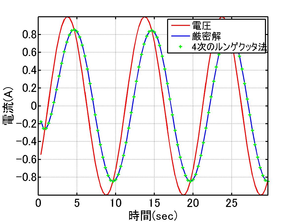
plot(t,i1,'r-','linewidth',2);
hold on
plot(t,i2,'b-','linewidth',2);
hold on
plot(t,i3,'g+','linewidth',2);
hold on
grid on
xlabel('時間(sec)','Fontsize',18)
ylabel('電流(A)','Fontsize',18)
h=legend('電圧',...,
'厳密解',...,
'4次のルンゲクッタ法',...,
1);
set(h,'FontSize',15)
axis([0 Inf -Inf Inf]);
h=gca
get(h)
set(h,'LineWidth',2,...,
'FontSize',18)
print -djpeg rungekutta4_method.jpg
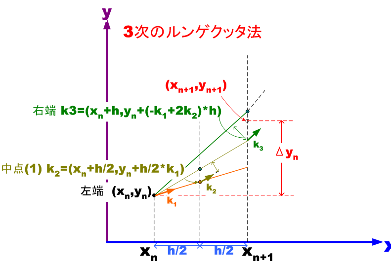
=f(x_n , y_n )") (1-1)
(1-1)=f(x_n+\frac{h}{2},y_n+\frac{h}{2}*k1(n))") (1-2)
(1-2)=f(x_n+h,y_n +(-k1(n)+ 2k2(n))*h)") (1-3)
(1-3)
 + 4k2(n) + k3(n) )*h") (1-4)
(1-4)
#include "stdafx.h"
#include<iostream>
#include<fstream>
#include<io.h>
#include<math.h>

#define PI 3.1415926

const static double Em=1.0;                              //電圧源
const static double R=1.0;                               //抵抗
const static double L=1.0;                               //コイル
const static double freq=0.1;                            //周波数0.1Hz
const static double omega=2*PI*freq;                     //角周波数
const static double theta=-PI/4.0;
const static double phi=atan(omega*L/R);
const static double tau = L/R;                           //時定数
const static double dh=(1/freq)/30.;                     //1周期の30分割
const static double Im=1.0/sqrt(R*R+(omega*L)*(omega*L));

double func1(double t,double cur);
double rungeKutta4zi(double t,double i4);

int _tmain(int argc, _TCHAR* argv[])
{

	errno_t err;
	FILE *fp_output;

	//変数
	double t=0;          //実時間
	double e=0;          //初期電圧
	double i1=0.0;       //初期電流(厳密解)
 	double i4=0.0;       //初期電流(4次のルンゲクッタ法)
	double i3=0.0;       //初期電流(3次のルンゲクッタ法)


	if( err = fopen_s(&fp_output,"renritu_bibun_kekka.txt","w")  != 0){ exit(2);}

	t=0;
	for(int n=1; n< 3*(int)((1/freq)/dh); n++){


		i4=rungeKutta4zi(t,i4);
 		i3=rungeKutta4zi(t,i3);
		//n=1から始まるから t=n*dh(n=1,2,3...)
		t=(double)n*dh;

		//電源電圧
 		e=Em*sin(omega*t+theta);
		//理論値電流
 		i1=Im*(sin(omega*t+theta-phi)-exp(-t/tau)*sin(theta-phi));

		printf("t = %f e=%f i1 = %f i3 = %f i4 = %f\n",t,e,i1,i3,i4);
 		fprintf_s(fp_output,"%f %f %f %f %f\n",t,e,i1,i3,i4);
	}

	if(fp_output != NULL) fclose(fp_output);
	getchar();
	return 0;
}


double rungeKutta4zi(double t,double i4){

	double k[4]={0,0,0,0};
	//これは t=n*dh(n=1,2,3,...)の計算となる
 	k[0]=func1(t,i4);
	k[1]=func1(t+dh/2,i4+dh/2*k[0]);
	k[2]=func1(t+dh/2,i4+dh/2*k[1]);
	k[3]=func1(t+dh,i4+dh*k[2]);

	i4=i4+(1./6.)*(k[0]+2*k[1]+2*k[2]+k[3])*dh;

	return i4;
}

double rungeKutta3zi(double t,double i3){

 	double k[4]={0,0,0,0};
 	//これは t=n*dh(n=1,2,3,...)の計算となる
	k[0]=func1(t,i3);
	k[1]=func1(t+dh/2,i3+dh/2*k[0]);
	k[2]=func1(t+dh,(-k[0]+2*k[1])*dh);

	i3=i3+(1./6.)*(k[0]+4*k[1]+k[2])*dh;

	return i3;
}

double func1(double t,double cur){

	double calcCur=(sin(omega*t+theta)-R*cur)/L;
	return calcCur;
}
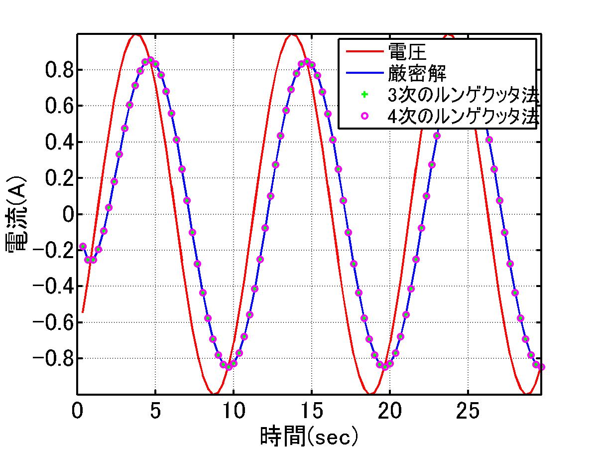
%%%%%%%%%%%%%%%%%%%%%%%%%%%%%%%%%%%%%
% 3 4次のルンゲクッタ法
%
%%%%%%%%%%%%%%%%%%%%%%%%%%%%%%%%%%%%
echo off
clear all
close all

load 'renritu_bibun_kekka.txt'

t=renritu_bibun_kekka(:,1);
v1=renritu_bibun_kekka(:,2);
ir=renritu_bibun_kekka(:,3);
i3=renritu_bibun_kekka(:,4);
i4=renritu_bibun_kekka(:,5);

plot(t,v1,'r-','linewidth',2);
hold on
plot(t,ir,'b-','linewidth',2);
hold on
plot(t,i3,'g+','linewidth',2);
hold on
plot(t,i4,'mo','linewidth',2);
hold on

grid on

xlabel('時間(sec)','Fontsize',18)
ylabel('電流(A)','Fontsize',18)

h=legend('電圧',...,
'厳密解',...,
'3次のルンゲクッタ法',...,
'4次のルンゲクッタ法',...,
1);
set(h,'FontSize',15)

axis([0 Inf -Inf Inf]);
h=gca
get(h)
set(h,'LineWidth',2,...,
'FontSize',18)

print -djpeg rungekutta4and3_method.jpg