") �̌`�ŕ\����Ă���Ƃ��̐ϕ��l�����߂�
�̌`�ŕ\����Ă���Ƃ��̐ϕ��l�����߂�
(1)�u�d�C�E�d�q�H�w�̂��߂̐��l�v�Z�@����v���{�C���@�����d�q�o�Ŏ�
(2)�u�f�B�W�^���M�������Z�p�v�ʈ䓿�݂��A�������A���c�O�A���C���� ���oBP��
(3)�u�悭�킩��L���v�f�@�v���X�h���� Ohmsha
http://szksrv.isc.chubu.ac.jp/java/physics/rlc/rlc0.html
http://www.asahi-net.or.jp/~jk2m-mrt/kiso_RLC.htm
http://ja.wikipedia.org/wiki/%E4%B8%89%E8%A7%92%E9%96%A2%E6%95%B0
http://www.cmplx.cse.nagoya-u.ac.jp/~furuhashi/education/CircuitMaker/chap1.pdf
http://www.akita-nct.ac.jp/~yamamoto/lecture/2003/5E/lecture_5E/diff_eq/node2.html
http://chemeng.on.coocan.jp/cemath/cemath08.html
http://homepage3.nifty.com/skomo/f6/hp6_3.htm
http://homepage1.nifty.com/gfk/rungekutta.htm
(a) �����̐���
�����������̉������߂�
(b) �����������̉��𐔒l�v�Z�ŋ��߂�
(c) �ϕ��̐���
(d) ���������̌`�̌`�ŕ\����Ă���Ƃ��̐ϕ��l�����߂�
(��ʓI�ɐ��l�ϕ�������Ӗ��́A�����̂��ω��̎�(�Ⴆ�Α��x�̊�)�Ȃǂŕ\����Ă���Ƃ�
���鎞�����玞���܂ł̋��������߂����Ƃ��ȂǂŎg�p�����B
������̕ω��̎����A��v�Z�ɂ���Čv�Z�\�Ȃ�ΐϕ��ɂ���Ď��ԂƋ����̊W�o��
���̎��Ԃ����邱�ƂŒ��ڋ��������ق��������B
�������A��ʓI�Ɏ��ԂƋ����̊W�̂悤�Ȏ����̂����o���邱�Ƃ��s�\�ȏꍇ�����̒��ɂ͑���
���ԂƑ��x�̊W�̂悤�ȕω��̎��������o�����Ƃ̕����e�ՂȂ̂����A�������v�Z�Őϕ����邱��
�͔��ɓ�����ߐ��l�ϕ�����Ă��ꂽ)
�}1-1 �ϕ������
��") ��
�� ����
���� �܂ł̐ϕ��́A
dx") (1-1)
(1-1)
�ŕ\����܂��B
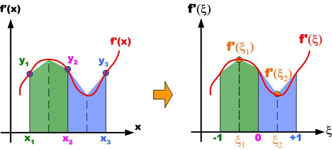
�K�E�X���W�����h���@�Ƃ́A���}�� ����
���� ��
�� ���W��
�E�}�̂悤��-1����1�܂ł� ���W�ɍ��W�ϊ����Đϕ������@�ł���B
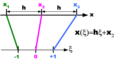
�}1-2 ���W�ϊ�
x���W���� ���W���̕ϊ����́A
 = h\xi + x_2") (1-2)
(1-2) (1-3)
(1-3)
�ƂȂ�A
�}1-1 �ϕ������
(1-1)���́A
dx = \int^{+1}_{-1}f'(x(\xi))hd\xi") (1-4)
(1-4)
�ƂȂ�B
(1-4)���́A (�E�F�C�e�B���O�|�C���g)���g�p����
)hd\xi \simeq h\sum^2_{i=1} f(\xi_i)w_i") (1-5)
(1-5)
�ƕ\�����B
�T���v�����O�|�C���g��2�̏ꍇ�A
�T���v�����O�|�C���g �ƃE�F�C�e�B���O�|�C���g
 �́A
�́A
�\1-1 2�_�K�E�X�E���W�����h���̌W��
| i | \xi_i | w_i |
|---|---|---|
| 1 | -0.577350 | 1.000000 |
| 2 | 0.577350 | 1.000000 |
�ƂȂ�B
2�_�̂Ƃ��̃T���v�����O�|�C���g�A�E�F�C�e�B���O�|�C���g�̌��ߕ��͕ʓr���Ђ��Q�l��
�����������B
�����ł́A�ǂ̂悤�ȋȐ��ł����W�ϊ����邱�Ƃ�-1����1�܂ł̐ϕ��ɗ��Ƃ����ނ��Ƃ��ł���
�����Ă��̐ϕ��̌v�Z���@�́A�\1-1�̃T���v�����O�|�C���g�ł̋Ȑ��̒l�ƃE�F�C�e�B���O�|�C���g��
�����āA�������킹�邱�ƂŊȒP�ɐϕ����v�Z���邱�Ƃ��ł���Ƃ����_�ł���B
�����قǂ̑�`�@�A�V���v�\���@�ɔ�ׂ�2�_���v�Z���邾���Őϕ������߂���_�����ɖ��͓I�ł���B
���x���グ�邽�߂ɂ̓T���v�����O�|�C���g�𑝂₵�Ă����悢���A���̏ꍇ�̃T���v�����O�|�C���g��
������E�F�C�e�B���O�|�C���g�͌��܂��Ă���̂ŕʓr���̎Q�l���Ђ��Q�l�̂��ƁB
��v�Z�ōs���Ă݂�B
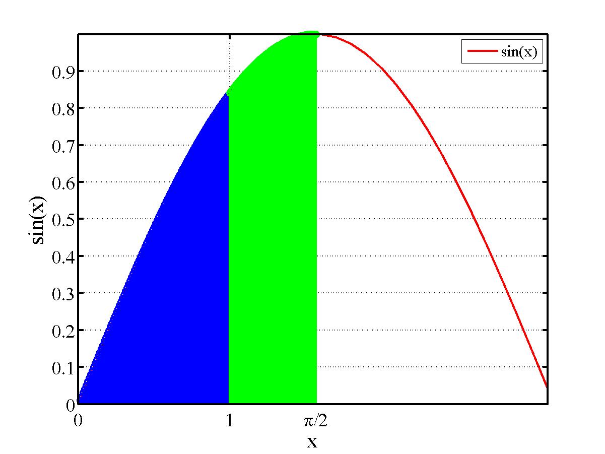
�܂��̈��
0����1�܂ł�̈�@ 1����pi/2�܂ł�̈�A
�Ƃ��A���ꂼ���ϕ����đ������킹�邱�ƂŐϕ����v�Z����B
�̈�1�̑S�̒���1�Ȃ̂�
h=1/2=0.5
x1=0
x2=0.5
x3=1
�ƂȂ�B
(a) �K�E�X���W�����h���@��K�p���� ,
, ���v�Z����B
 = h\xi_1 + x_2")
 = 0.5*(-0.577350) + 0.5")
 = 0.211325")
 = h\xi_2 + x_2")
 = 0.5*(0.577350) + 0.5")
 = 0.7887")
(b) (a)������sin(x)�ɑ������)") �����߂�B
�����߂�B
)=f(0.211325)=\sin(0.211325)=0.2098")
)=f(0.7887)=\sin(0.7887)=0.7094")
(c) w_i") ���v�Z����
���v�Z����
)w_1 + f(x(\xi_2))w_2 = 0.2098+0.7094=0.9192")

�̈�1�́A
h= (pi/2 - 1)/2  = 0.5708/2 = 0.2854
x1=1
x2=1.2854
x3=1.5708
�ƂȂ�B
(a) �K�E�X���W�����h���@��K�p���� ,
, ���v�Z����B
 = h\xi_1 + x_2")
 = 0.2854*(-0.577350) + 1.2854")
 = 1.1206")
 = h\xi_2 + x_2")
 = 0.2854*(0.577350) + 1.2854")
 = 1.4502")
(b) (a)������sin(x)�ɑ������)") �����߂�B
�����߂�B
)=f(1.1206)=\sin(1.1206)=0.9004")
)=f(1.4502)=\sin(1.4502)=0.9927")
(c) w_i") ���v�Z����
���v�Z����
)w_1 + f(x(\xi_2))w_2 = 0.9004+0.9927=1.8931")

0.4596+0.5403=0.9999
%%%%%%%%%%%%%%%%%%%%%%%%%%%%%%%%%%%%%
% �K�E�X�E���W�����h���@
%
%%%%%%%%%%%%%%%%%%%%%%%%%%%%%%%%%%%%
echo off
clear all
close all
y=[];
x=[];
for i=0:0.1:pi
x=[x,i];
y=[y,sin(i)];
end
area1x=[];
area1y=[];
for i=0:0.01:1
area1x=[area1x,i];
area1y=[area1y,sin(i)];
end
area2x=[];
area2y=[];
for i=1:0.01:pi/2
area2x=[area2x,i];
area2y=[area2y,sin(i)];
end
plot(x,y,'r-','linewidth',2);
hold on
stem(area1x,area1y,'bo','linewidth',2);
hold on
stem(area2x,area2y,'go','linewidth',2);
grid on
% x���x���Ƃ��̕����̑傫���A���̑����̐ݒ�
str={'0','1','p/2','p'}
set(gca,'FontName','symbol','xtick',[0,1,pi/2,pi],'xticklabel',str)
set(gca,'LineWidth',2,'FontSize',18)
% x-y�͈�
axis([-Inf Inf -Inf Inf]);
% x���x���Ay���x��
xlabel('x','Fontsize',20,'FontName','Times');
ylabel('sin(x)','Fontsize',20,'FontName','Times')
h=legend('sin(x)',...,
1);
set(h,'FontSize',15,'FontName','Times')
print -djpeg sin_sekibun_gause_rugendol_byouga.jpg
 �����
�����![[0,1]](BFF4C3CDB7D7BBBB40BFF4C3CDC0D1CAAC40A4BDA4CE3340A5ACA5A6A5B9A5EBA5B8A5E3A5F3A5C9A5EBCBA1_eq0047.gif "[0,1]") �ɂ�����Gauss-Legendre�@��p���ĉ����B
�ɂ�����Gauss-Legendre�@��p���ĉ����B3.141588 3.141593 3.147541
// gauss-legendre-CVer.cpp : �R���\�[�� �A�v���P�[�V�����̃G���g�� �|�C���g���`���܂��B
//
#include "stdafx.h"
#include "stdafx.h"
#include<iostream>
#include<fstream>
#include<io.h>
double sympson_method(double (*function)(double x),double a,double b,int num);
double daikei_method(double (*function)(double x),double a,double b,int num);
double gauss_legendre_method(double (*function)(double x),double a,double b);
double func(double x);
int _tmain(int argc, _TCHAR* argv[])
{
errno_t err;
FILE *fp_output;
double ans_sympson=0.;
double ans_daikei=0.;
double ans_gauss_legendre=0.;
if( err = fopen_s(&fp_output,"gause_legendre_value.txt","w") != 0){ exit(2);}
double a=0.;
double b=1.0;
int n=200;
double h2 = (b-a)/(double)n;
double h=h2/2.;
ans_daikei = daikei_method(&func,a,b,n);
ans_sympson = sympson_method(&func,a,b,n);
ans_gauss_legendre = gauss_legendre_method(&func,a,b);
fprintf_s(fp_output,"%f %f %f\n",ans_daikei,ans_sympson,ans_gauss_legendre);
printf("%f %f %f\n",ans_daikei,ans_sympson,ans_gauss_legendre);
if(fp_output != NULL) fclose(fp_output);
getchar();
return 0;
}
//�ϕ��͈̔�[a,b]�Ƃ��͈̔͂̕�����num
double gauss_legendre_method(double (*function)(double x),double a,double b){
double w1=1.;
double w2=1.;
double xi1=-0.577350;
double xi2= 0.577350;
double h=(b-a)/2.;
double x1=a;
double x2=a+h;
double x3=b;
double x_xi1=h*xi1 + x2;
double x_xi2=h*xi2 + x2;
double ans1=0.;
double ans2=0.;
double ans=0.;
ans1=(*function)(x_xi1);
ans2=(*function)(x_xi2);
ans = h*(ans1*w1 + ans2*w2);
return ans;
}
//�ϕ��͈̔�[a,b]�Ƃ��͈̔͂̕�����num
double sympson_method(double (*function)(double x),double a,double b,int num){
//�ϕ��͈̔͂Ƃ��͈̔͂����鐔num���狁�߂��闣�U�Ԋu
double h=0.;
double h2=0.;
//�V���v�\���@�Ŏg����ϐ�
double ans=0;
double term1=0.;
double term2=0.;
double term3=0.;
double term4=0.;
h2 = (b-a)/(double)num;
h=h2/2.;
ans=0.;
term1=0.;
term2=0.;
term3=0.;
term4=0.;
///// ��������sympson�@ ///////////////
//��1���̌v�Z
term1=(*function)(a);
//��2���̌v�Z y2+y4+y6+.....+y_{2n-2}
for(int i=2;i<=(2*num-2);i=i+2){
term2=term2+(*function)(a+i*h);
}
//��3���̌v�Z y1+y3+y5+....+y_{2n-1}
for(int i=1;i<=(2*num-1);i=i+2){
term3=term3+(*function)(a+i*h);
}
//��4���̌v�Z
term4=(*function)(b);
ans=h/3.*(term1+2*term2+4*term3+term4);
return ans;
}
//�ϕ��͈̔�[a,b]�Ƃ��͈̔͂̕�����num
double daikei_method(double (*function)(double x),double a,double b,int num){
double h = (b-a)/(float)num;
double ans=0;
for(int i=1;i<=num;i++){
ans=ans+(*function)(a+(i-1)*h)+(*function)(a+(i*h)) ;
}
return ans=h/2.*ans;
}
double func(double x){
double y;
y=4.0/(1.0+x*x);
return y;
}